Sumif Date Range Can Be Fun For Anyone

If "blank" indicates cells that include absolutely nothing - no formula, no absolutely no size string returned by some other Excel function, after that make use of "=" as the standards, like in the complying with SUMIF formula: =SUMIF(A 2: A 10,"=", C 2: C 10) If "blank" includes absolutely no size strings (as an example, cells with a formula like =""), then utilize "" as the standards: =SUMIF(A 2: A 10,"", C 2: C 10) Both of the above solutions evaluate cells in column An and also if any vacant cells are located, the equivalent values from column C are included.

Usually, you utilize the SUMIF feature to conditionally sum worths based on dates in the same method as you utilize message as well as numeric criteria. If you desire to sum worths representing the dates that are higher than, less than or equivalent to the day you specify, after that make use of the Standard Formula Instance Description Amount worths based on a specific date.

Amount values if a matching day is better than or equal to an offered day. =SUMIF(B 2: B 9,">=10/29/2014", C 2: C 9) Amount worths in cells C 2: C 9 if a corresponding day in column B is better than or equal to 29-Oct-2014. Amount values if an equivalent date is above a date in another cell.

In case you wish to sum worths based upon a current date, then you need to use Excel SUMIF in mix with the TODAY() feature as demonstrated listed below: Standard Solution Instance Sum values based on the existing day. =SUMIF(B 2: B 9, TODAY(), C 2: C 9) Amount values matching to a prior day, i.e.

The Main Principles Of Sumif Multiple Criteria

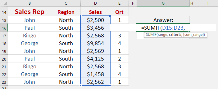
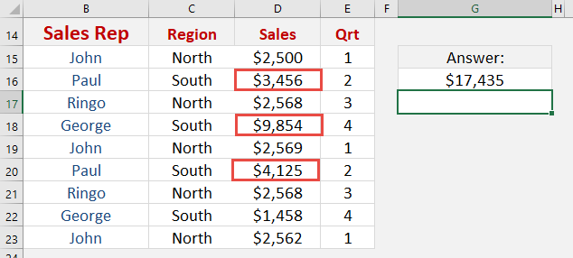
=SUMIF(B 2: B 9, "" & TODAY(), C 2: C 9) Sum values if a day occurs in a week( i.e. today +7 days).=SUMIF (B 2: B 9, "="& TODAY( )+7, C 2: C 9) The screenshot below highlights how you can make use of the last formula to locate the total amount of all items that ship in a week. In Excel 2007 and also greater, you can additionally use the SUMIFS feature that permits multiple standards, which is also a far better option. While the last is the subject of our next article, an example of the SUMIF formula complies with below: =SUMIF(B 2: B 9, ">=10/1/2014", C 2: C 9) - SUMIF(B 2: B 9, ">=11/1/2014", C 2: C 9) This formula summarize the worths in cells C 2: C 9 if a day in column B is between 1-Oct-2014 as well as 31-Oct-2014, comprehensive.

The first SUMIF feature accumulates all the cells in C 2: C 9 where the corresponding cell in column B is more than or equal to the beginning date (Oct-1 in this example). Then you simply have to deduct any values that fall after the end day (Oct-31), which are returned by the second SUMIF feature.

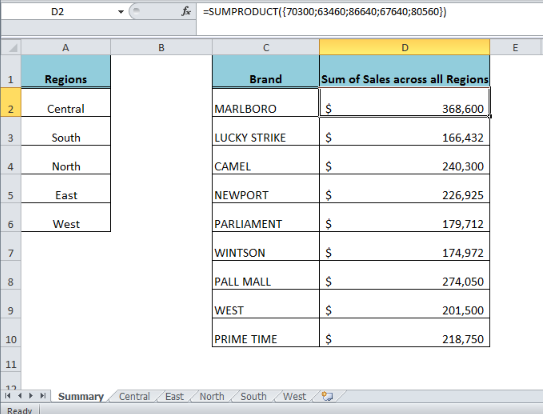
Intend, you have a summary table of regular monthly sales. Given that it was combined from a numbers of regional reposts, there are a few records for the same product: So, exactly how do you locate the overall of apples sold in all the states in the previous 3 months? As you bear in mind, the measurements of sum_range are figured out by the dimensions of the array parameter.

This is not what we are seeking, right? The most logical and easiest remedy that recommends itself is to produce an assistant column that computes private sub-totals for every row and afterwards recommendation that column in the sum_range criteria. Go in advance as well as place a simple SUM formula in cell F 2, after that fill up down column F: =SUM(C 2: E 2) After that, you can create a common SUMIF formula such as this: =SUMIF(A 2: A 9, "apples", F 2: F 9)or=SUMIF(A 2: A 9, H 1, F 2: F 9) In the above solutions, sum_range is specifically of the very same dimension as array, i.e

Getting The Sumif Vs Sumifs To Work

. There could be numerous reasons that Excel SUMIF is not helping you. In some cases, your formula does not return what you anticipate only because the data key in a cell or in some disagreement isn't matched for the SUMIF feature. So, right here is a checklist of points to examine. The very first (variety) and 3rd (sum_range) criteria of your SUMIF formula have to constantly be an array referral like A 1: A 10.

Proper formula: =SUMIF(A 1: A 3, "blossom", C 1: C 3) Wrong formula: =SUMIF( 1,2,3, "flower", C 1: C 3) As almost any type of other Excel function, SUMIF can reference various other sheets and also workbooks, given they are presently open. For instance, the adhering to formula will sum the values in cells F 2: F 9 in Sheet 1 of Book 1 if an equivalent cell in column A if the same sheet includes "apples": =SUMIF( [Reserve 1. xlsx] Sheet 1!$A$ 2:$A$ 9,"apples", [Schedule 1. xlsx] Sheet 1!$F$ 2:$F$ 9) Nevertheless, this formula will not work as quickly as Book 1 is closed.

As kept in mind in the start of this tutorial, in modern variations of Microsoft Excel, the range and also sum_range parameters does not need to be similarly sized. In Excel 2000 and also older, unequally sized variety as well as sum_range can cause problems. Nevertheless, also in one of the most recent variations of Excel 2010 and Excel 2016, complicated SUMIF formulas where sum_range has much less rows and/or columns than array are picky.

If you have actually occupied your workbook with complex SUMIF solutions that decrease your Excel, check out The Excel SUMIF instances explained in this tutorial only touch on a few of the standard uses of this function. In the next write-up, we'll check out advanced solutions that harness the actual power of SUMIF as well as SUMIFS and also let you amount by multiple criteria.

The Best Strategy To Use For How To Use Sumif

I intend to do an amount of cells, with multiple criterias. I have found out that the way to do it is with sumproduct. Such as this =SUMPRODUCT((A 1: A 20="x")*(B 1: B 20="y")*(D 1:D 20)) The trouble I am having is that the A row includes merged cells (which I can not transform) In my situation I want to do an amount of every number in the provided row under both 2010 and also 2011 meeting my standards.

excel sumif criteria not equal excel sumif criteria range excel sumif horizontal